Electronic compass dynamic heading error correction

Analog Output-Full Attitude Three-Dimensional Electronic Compass

Electronic compass is a navigation and positioning device that uses the geomagnetic field to obtain heading (azimuth) angle information. Thanks to the development of sensors and semiconductor technology, electronic compasses have achieved miniaturization and micro-power consumption, and can compensate for sensor errors and external magnetic interference by using appropriate signal conditioning circuits and data processing algorithms. In order to improve the heading accuracy of compasses, its error correction and compensation methods have been fully studied in recent years. However, commonly used correction methods such as the multi-position method and the ellipsoid fitting method do not consider the dynamic response characteristics of the sensor. To address this shortcoming, we performed dynamic modeling and error correction on the three-axis magnetometer in the digital compass.

1.Overview of electronic compass

It usually uses accelerometers and magnetometers to measure gravity acceleration and geomagnetic field vectors respectively, and then calculate three Euler angles such as heading angle ψ, pitch angle θ and roll angle φ based on gravity and geomagnetic field vectors, which are used to describe their carrier posture. Assume that the x-axis, y-axis and z-axis of the carrier coordinate system point to the front, right and bottom of the carrier in sequence, while the three axes of the reference coordinate system point to the north, east and ground in sequence. Rotate the reference system around its x-axis by φ, its y-axis by θ, and its z-axis by ψ, then it will coincide with the carrier system. On the other hand, since the gravity vector g is vertically downward and the horizontal component of the geomagnetic field vector h points to magnetic north, the roll angle φ, pitch angle θ and magnetic heading angle ψ can be calculated sequentially from the measured values of these two vectors in the carrier system.

2 Dynamic Characteristics Modeling and Correction

2.1 Dynamic response model

The dynamic characteristics of sensors are often described by transfer functions. The transfer function is usually defined in the complex frequency domain, that is, the s domain, and is closely related to time constants, natural frequencies, damping ratios and other indicators. However, in an digital compass, the output signal of the magnetometer is first processed through analog-to-digital conversion, so it is more convenient to perform dynamic modeling in the discrete domain, that is, the z domain. In addition, the traditional system identification method is to first fit the sensor transfer function H(s) =Y(s)X (s), where X (s) and Y(s) are the Laplace transform of the input and output signals respectively, Then take corresponding compensation measures according to H (s). In order to simplify the correction and compensation process, this article directly fits the inverse function of the transfer function, that is, D(z)=h(z)v(z) in fitting equation (1), where h(z) and v (z) are the z-transform of the true value of the magnetic field and the magnetometer output sequence respectively.

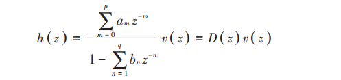
Record the true value of the magnetic field and the magnetometer output corresponding to the sampling time k as hk and vk respectively, then equation (1) can be changed to

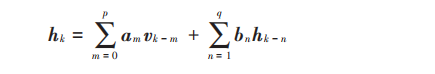
When using equation (2) to perform magnetometer dynamic modeling and error compensation, the following points should be noted:

1) Since hk and vk are both three-dimensional vectors, the coefficients am and bn should both be in the form of 3×3 matrices;

2) In order to ensure numerical stability and reduce computational complexity, the orders p and q should not be too high. Here we take p=2 and q=1;

3) In order to compensate for the constant error of the magnetometer (including zero error and hard magnetic interference), the constant term c should be added to equation (2).

Considering the above factors, equation (2) can be further rewritten as equation (3):

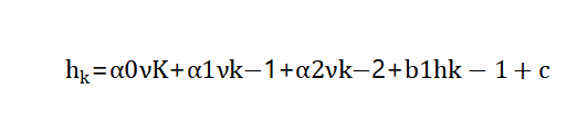
Equation (3) is the magnetometer dynamic error compensation model, in which a0~a2 and b1 are all 3×3 matrices, c is a three-dimensional constant vector, with a total of 39 parameters.

2.2 Data collection and correction

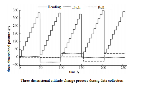
In order to accurately fit the parameters in equation (3) and ensure the static and dynamic accuracy of digital compass after correction, the data collection process should adopt a combination of dynamic and static methods, that is, sufficient data should be collected under both static and dynamic conditions. Consider a simple and commonly used data collection method in the ellipsoid fitting method: place the compass horizontally and tilted forward, backward, left, and right in five states, and rotate it around the vertical axis in these five states. week. On this basis, by selecting several orientations as static points during the rotation, a data collection process that combines dynamic and static data can be formed.

3 Calibration experiment

3.1 Experimental methods

We use the magnetometer's three-axis electronic compass for calibration experiments, and use the attitude module to provide accurate heading, pitch and roll angle data as a reference.

The experimental steps are as follows:

1) Original data collection

2) The multi-position method, the ellipsoid fitting method and the compensation method based on the dynamic model proposed by us are used to correct and compensate the error of the electronic compass;

3) After using the above three methods for compensation, check the static accuracy and dynamic accuracy of the heading angle of the electronic compass.

3.2 Experimental results

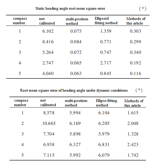
In the experiment, a total of five digital compasses were subjected to error compensation and accuracy testing according to the above steps. The root mean square error (RMSE) of heading angle under static and dynamic conditions are listed in Table 1 and Table 2 respectively.

3.3 Experimental conclusions

It can be seen from Table 1 and Table 2 that the results of the three calibration methods used in the experiment have good repeatability. In addition, by comparing the measurement results without correction and after correction by each method, the following conclusions can be drawn.

First of all, no matter what method of correction is used (including uncorrected time), the dynamic error of each electronic compass used in the experiment is greater than the static error, indicating that the dynamic response characteristics of the magnetometer have a non-negligible impact on the heading angle accuracy. Secondly, after correction using the multi-position method or ellipsoid fitting method, the heading accuracy is better under static conditions (and the multi-position method is better than the ellipsoid fitting method), but the heading angle error is still large under dynamic conditions. In other words, these two methods can only guarantee the static accuracy of the compass. In contrast, our method significantly improves both the static and dynamic accuracy of the compass. The static heading error (RMSE) can be reduced to within 0.5°, and the dynamic heading error can be reduced to within 2.5°. Compared with the multi-position method and the ellipsoid fitting method, the method in this paper improves the dynamic accuracy by more than 50%. It can be seen from Figure 2.

4 Summary

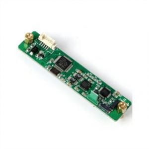
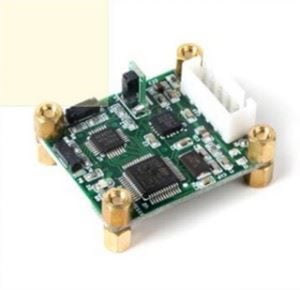
In view of the shortcoming that traditional correction methods cannot compensate for the dynamic error of digital compasses, we modeled the dynamic characteristics of a three-axis magnetometer and used the model to conduct error correction and compensation experiments on digital compass, which proved the feasibility of this method. Of course, after correction by this method, the dynamic heading angle error can be reduced to less than 2.5° (RMS), and the static error can be guaranteed to be less than 0.5° (RMS), which significantly improves the dynamic accuracy of compass. For Ericco's ER-EC-360A and ER-EC-365V, we can use the above-mentioned error correction methods and compensation experiments to further improve the dynamic accuracy of the electronic compass.