Performance Analysis of GNSS RTK Timing

Timing services are an indispensable part of national economy and people's livelihood. Currently used timing methods include shortwave timing, longwave timing, internet timing, telephone timing, fiber-optic timing, and GNSS timing. Among these methods, GNSS RTK timing stands out for its high accuracy, simplicity of implementation, and outstanding application potential in short-distance precision timing and time synchronization without relying on real-time precise ephemeris. This paper primarily utilizes observation data from three GNSS tracking stations of the National Time Service Center of the Chinese Academy of Sciences, focusing on BDS-3, GPS, and Galileo, to analyze RTK timing accuracy, convergence time, and stability.

Backgroundof RTK Timing

Global satellite navigation systems mainly include GPS, GLONASS, Galileo, BDS, etc., providing positioning, navigation, and timing services (PNT) to global users. Timing is a fundamental service provided by GNSS, achieved through the transmission of time via GNSS space signals (SIS). It has a wide coverage, minimal propagation attenuation, and is not limited by the number of users. GNSS timing is widely used in time synchronization for military digital communication networks, telecommunication networks, power systems, and more.

The core of RTK timing is applying RTK positioning technology to timing. The mobile station receives real-time observation data from the reference station through a communication link, forms a differential with the local observation data, and solves the relative clock difference between the mobile station and the reference station. When the reference station is connected to the standard time frequency signal UTC(k) in the timing laboratory, the RTK timing solution for clock difference is the relative clock difference of the mobile station's clock relative to standard time, achieving the purpose of timing.

Current research on the timing mainly focuses on single systems such as GPS and BDS-3, with limited reports on the research of GNSS multi-system fusion RTK timing. To better verify the performance of GNSS multi-system fusion RTK timing and enhance reliability in urban environments, this paper first presents the observation equations for multi-system RTK timing. Subsequently, experiments are conducted using observation data from GPS, BDS-3, and Galileo based on the time-frequency resources of the National Time Service Center, analyzing GNSS multi-system fusion RTK timing from the aspects of timing accuracy, convergence time, and stability.

Multi-GNSS RTK Timing Principle and Model

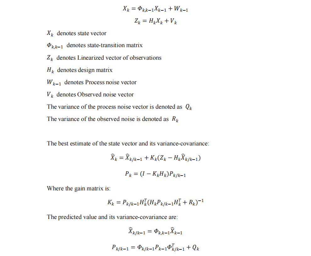
The principle of RTK timing is similar to RTK positioning. The user receiver receives real-time pseudorange and carrier phase observation data from the reference station through a communication link, forms inter-station differential measurements with the user receiver, and solves the user receiver's clock error and three-dimensional coordinates. When the distance between two measurement stations is short, the impact of ionospheric delay and tropospheric refraction has strong correlation, making single-differencing capable of eliminating most of the atmospheric refraction errors. In multi-system RTK timing, using the GPS system's clock error as a reference, the system inter-bias (ISB) of other systems introduced relative to GPS is considered. The parameter estimation for the timing is carried out using an extended Kalman filter, and the simplified observation equation can be expressed as:

Performance Analysis of GNSS RTK Timing-equation

3. Specific Analysis of RTK Timing Performance

The following specific analysis is based on the modified RTKLIB software. Short baseline multi-system single-frequency and dual-frequency RTK timing experiments are conducted with SE22 and XIA6 as mobile stations, and SEPT as the reference station. The experiments involve kinematic, static, and fixed station coordinates timing modes.

3.1 Timing Accuracy

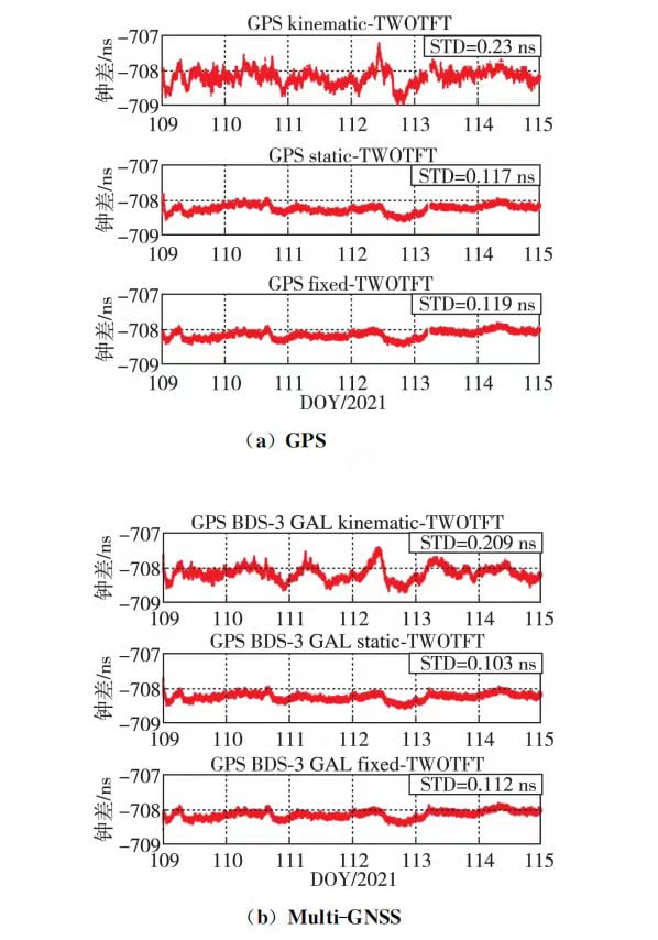
Differences between SE22 single-frequency RTK timing, dual-frequency, and optical fiber two-way time-frequency transfer results are shown in Figures 1 and 2. The figures represent GPS single system (a) and multi-system (b). From the timing difference graphs, it can be observed that there is an absolute error of -708 ns between the two timing methods. This is mainly caused by the delay in the external time signal of SEPT and SE22 receivers in timing. Without considering the convergence process, the peak-to-peak difference in single-frequency dynamic mode is less than 2 ns, and in single-frequency static and fixed station coordinate modes, as well as dual-frequency modes, the peak-to-peak difference is less than 1 ns.

Fig. 1 Differences between SE22 si ngle frequency RTK and optical fibre tworway time frequency transfer

Through calculations, in dynamic mode, the timing accuracy of single-frequency multi-system RTK is improved by 9.13% and 9.01% compared to GPS single system for the two baselines. In static mode, the improvement is 6.09% and 11.76%, and in fixed station coordinate mode, the improvement is 3.04% and 5.79%. The timing accuracy in dual-frequency dynamic mode is improved by 2.92% and 3.01%, in static mode by 4.65% and 2.41%, with almost no improvement in fixed station coordinate mode. Compared to optical fiber two-way time-frequency transfer, the standard deviation of timing difference in single-frequency RTK timing is better than 0.25 ns, and in dual-frequency mode, it is better than 0.15 ns. The improvement in timing accuracy is more pronounced in multi-system single-frequency timing compared to dual-frequency.

3.2 Convergence Time

To quantify the degree of reduction in convergence time for multi-system timing compared to GPS single system in dynamic and static modes, convergence time is indirectly characterized based on the precise coordinates of the mobile station. Convergence time is defined as the time required to solve three-dimensional directional positioning errors less than 1 dm and maintain them for at least 10 epochs. The average value of the convergence time for 12 dm is taken as the final convergence time, and the percentage reduction in convergence time for multi-system RTK timing compared to GPS single system is calculated, as shown in Figure 3. The yellow line in Figure 3 represents the percentage reduction in convergence time for multi-system compared to GPS single system. The abscissa includes K-S, S-S, K-D, and S-D, representing single-frequency dynamic mode, single-frequency static mode, dual-frequency dynamic mode, and dual-frequency static mode, respectively.

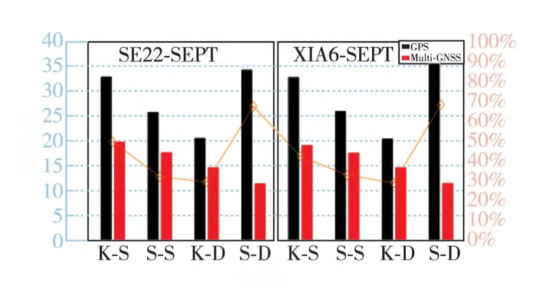
From Figure 3, it can be seen that the convergence time of GPS single system RTK timing is above 20 minutes, while the convergence time for multi-system is less than 20 minutes. The shortest convergence time for multi-system is in dual-frequency static mode, at 11.29 minutes. The convergence time for dynamic and static modes in multi-system RTK timing is significantly shorter than GPS single system, with a reduction of at least 25%. In static mode, the convergence time for dual-frequency RTK is reduced the most, with reductions of 66.9% and 67.8% for the two baselines. The fusion of multiple systems significantly increases the number of visible satellites, leading to a noticeable reduction in the convergence time of RTK timing.

3.3 Stability

The evaluation of time transfer stability commonly uses the method proposed by the American scholar D.W. Allan, namely the Allan variance. This method describes the fluctuation of frequency by calculating the average standard deviation of oscillator noise after multiple measurements. The frequency stability of inter-station clock differences in RTK timing is expressed in terms of modified Allan deviation (MDEV), as shown in Figures 4 and 5. Figures (a) represent single-frequency, and (b) represent dual-frequency. The frequency stability results of inter-station clock differences for all fixed station coordinate modes are presented as subplots in the lower-left corner of the main plot. The stability of multi-system RTK timing in three modes enters the range of 10^-15. In fixed station coordinate mode, the frequency stability of inter-station clock differences for multi-system RTK timing is almost identical to GPS single system.

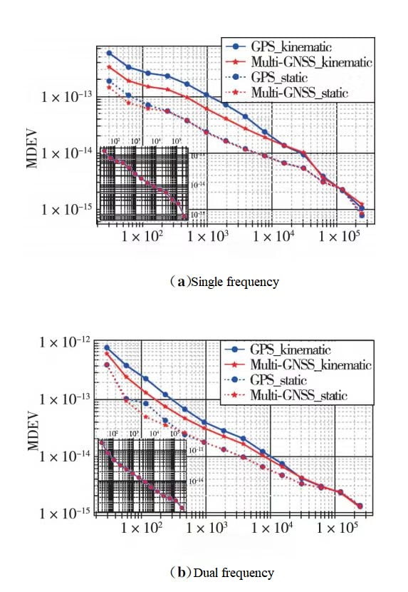
For single-frequency RTK timing, with an average time of 120 s, the frequency stability in dynamic mode is improved by 42.5% and 42.3% for the two baselines, and in static mode, it is improved by 13.8% and 14.2%. With an average time of 960 s, the improvements are 43.8% and 43.75% in dynamic mode, and 2.92% and 2.81% in static mode. For dual-frequency RTK timing, with an average time of 120 s, the improvements in dynamic mode are 43.44% and 42.09%, and in static mode, they are 42.12% and 27.18%. With an average time of 960 s, the improvements are 21.74% and 22.26% in dynamic mode, and 0.33% and 1.23% in static mode. The stability of multi-system RTK timing is significantly superior to GPS single system in dynamic mode and shows some improvement in static mode. In dynamic and static modes, the short-term stability of multi-system RTK timing improves to varying degrees compared to GPS single system, but as the average time increases, this improvement diminishes significantly.

4. Conclusion

Compared to GPS single system, multi-system GNSS significantly increases the number of observable satellites, leading to a significant improvement in the convergence speed and short-term stability of RTK timing in dynamic and static modes. Timing accuracy is also improved to a certain extent. Multi-system GNSS RTK timing demonstrates significant advantages in urban environments, improving timing accuracy, reducing convergence time, and exhibiting better frequency stability in the short term.

In practical applications, GNSS RTK timing is a promising GNSS solution, especially suitable for the high-precision and high-reliability time synchronization needs in urban environments. For example, ER-GNSS-M03, a new generation GNSS all-system multi-frequency high-precision timing module, with PPS accuracy of 2.5ns and RTK initialization time less than 5s. The cold start time for TTFF is less than 30s. Additionally, the module integrates filters, linear amplifiers, and features an optimized RF structure and interference suppression capability. It incorporates adaptive anti-interference technology and U-Auto Align multipath suppression technology, supporting interference detection and deception detection functions, ensuring the module delivers excellent performance in complex electromagnetic environments.

I will appreciate it if you find this article helps you a lot. For more information, please read the products below. Always feel free to contact us:

Email: info@ericcointernational.com